Point Mapping
SDS 192: Introduction to Data Science
Lindsay Poirier
Statistical & Data Sciences, Smith College
Fall 2022
For Today
- Quiz 2 Posted!
- Projections
- Coordinate Reference Systems
- Point Mapping in Leaflet
Why analyze spatial data?
- How are features distributed across geographies, and what does this tell us about potential disparities?
- Where are certain events or features concentrated, and what other conditions might implicate these patterns?
- What kinds of features are proximate, and what impact might this have?
- What is the best way to get from point A to point B?
Geographic Comparisons
Concentrations of Features
Where are the most were Missed Collections on October 1, 2021?
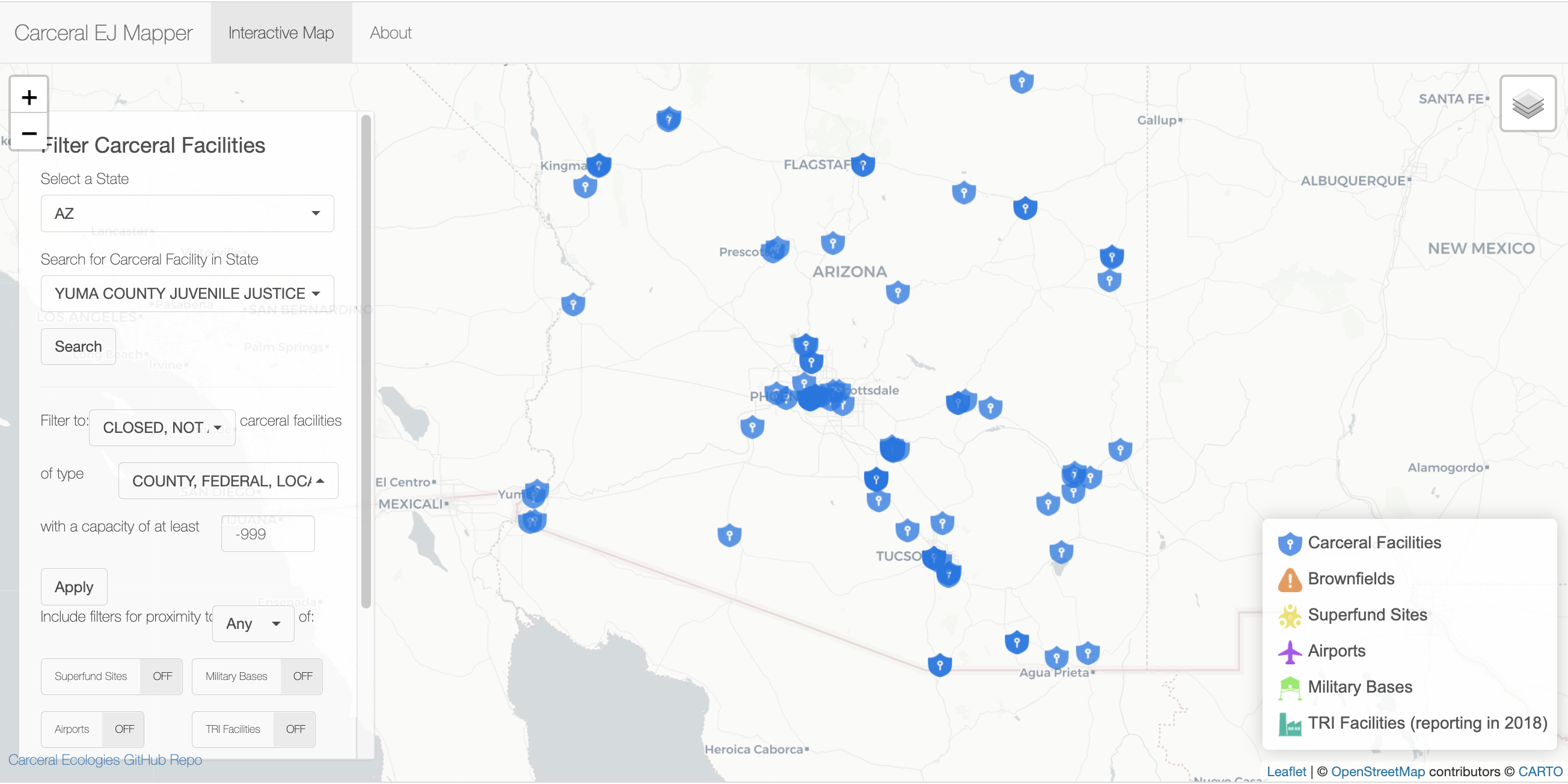
Proximity Analysis: Carceral EJ Mapper

Projections
- Means by which we convert curved surface of the globe to 2D rectangle
- Necessarily distorts the surface (e.g. area, distance)
- Many projections exist, serving different purposes

Strebe, Cylindrical Equal Area Projection

Strebe, Sinusoidal projection

Strebe, Goode’s homolosine projection
Strebe, Mercator projection
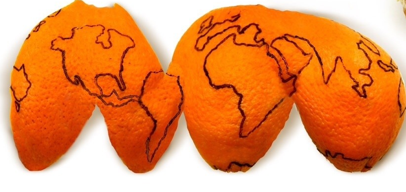
Orange Peel Example
- Imagine that you peel an orange
- Datum is the original shape of the fruit (e.g. orange, lemon, apple, grapefruit)
- Projection is how we go about peeling and flattening the orange

https://geohackweek.github.io/visualization/02-projections/
Coordinate Reference System (CRS)
- Points are in different locations depending on how we flatten Earth’s surface into 2D map
- CRS is a system for locating features on a certain map projection via coordinates
- Thousands of CRSs but some are more common than others (e.g. WGS 84 most common)
- For locations to appear correctly on maps, geographic features and underlying maps need to share same CRS
sf Package
- Encodes spatial data into geometry objects
- Locates latitudes and longitudes according to a particular CRS
- Enables setting and transforming CRSs
How do I know which to use?
- We pray that it’s listed somewhere in data documentation.
- Not always the case.
Leaflet
- Start by calling
leaflet()function, setting the original view, and adding basemap tiles - Note that you need to look up the coordinates of the geography you wish to center in on.
Adding Markers
addCircleMarkers()addMarkers()addPolygons
Transforming CRS
- Why didn’t points appear?
- Leaflet assumes that coordinates will be in
CRS:4326(WGS84) - We can use
st_transform()to convert points to a different CRS.
Leaflet, cont.
Layers
NYC Rodent and Litter Complaints on April 4, 2022
Creating Palettes for Points
colorNumeric(): Maps numbers to colors in a specified palettecolorBin(): Maps numbers into equally-spaced intervals (e.g. 0-10, >10-20, etc.)colorQuantile(): Maps numbers into equally-sized intervals (same number of observations in each grouping)colorFactor(): Maps categories into a specified number of categorical buckets